Contents:
Repeated Cross-fitting
The purpose of repeated cross-fitting is to reduce the variability of estimate based on a specific split of data by summarizing estimates using different splits as suggested by Chernozhukov (2018).
Create an AIPW object
library(AIPW)
library(SuperLearner)
#> Loading required package: nnls
#> Loading required package: gam
#> Loading required package: splines
#> Loading required package: foreach
#> Loaded gam 1.22-2
#> Super Learner
#> Version: 2.0-28.1
#> Package created on 2021-05-04
library(ggplot2)
set.seed(123)
data("eager_sim_obs")
cov = c("eligibility","loss_num","age", "time_try_pregnant","BMI","meanAP")

AIPW_SL <- AIPW$new(Y= eager_sim_obs$sim_Y,
                    A= eager_sim_obs$sim_A,
                    W= subset(eager_sim_obs,select=cov),
                    Q.SL.library = c("SL.glm"),
                    g.SL.library = c("SL.glm"),
                    k_split = 2,
                    verbose=TRUE)$
  fit()$
  summary()
#> Done!
#>                  Estimate     SE 95% LCL 95% UCL   N
#> Risk of Exposure    0.446 0.0474 0.35254   0.539 118
#> Risk of Control     0.287 0.0635 0.16249   0.411  82
#> Risk Difference     0.159 0.0790 0.00378   0.313 200
#> Risk Ratio          1.553 0.2441 0.96220   2.505 200
#> Odds Ratio          1.997 0.3625 0.98121   4.063 200
Decorate with Repeated class
# Create a new object from the previous AIPW_SL (Repeated class is an extension of the AIPW class)
repeated_aipw_sl <- Repeated$new(aipw_obj = AIPW_SL)
# Fit repetitively
repeated_aipw_sl$repfit(num_reps = 30, stratified = F)
# Summarise the median estimate, median SE, and the SE of median estimate adjusting for `num_reps` repetitions
repeated_aipw_sl$summary_median()
#>                  Median Estimate Median SE SE of Median Estimate
#> Risk of exposure           0.434    0.0500                0.0516
#> Risk of control            0.303    0.0596                0.0635
#> Risk Difference            0.130    0.0776                0.0856
#> Risk Ratio                 1.428    0.2211                0.2612
#> Odds Ratio                 1.765    0.3439                0.4350
#>                  95% LCL Median Estimate 95% UCL Median Estimate
#> Risk of exposure                  0.3333                   0.536
#> Risk of control                   0.1787                   0.428
#> Risk Difference                  -0.0373                   0.298
#> Risk Ratio                        0.9161                   1.940
#> Odds Ratio                        0.9122                   2.617
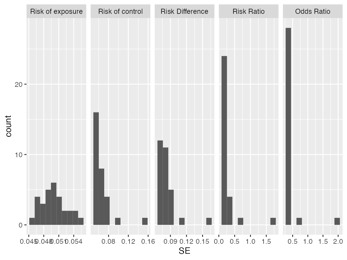
# Check the distributions of estiamtes from `num_reps` repetitions
s <- repeated_aipw_sl$repeated_estimates
ggplot2::ggplot(ggplot2::aes(x=Estimate),data = s) + ggplot2::geom_histogram(bins = 10) + ggplot2::facet_grid(~Estimand, scales = "free")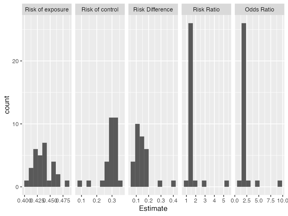
ggplot2::ggplot(ggplot2::aes(x=SE),data = s) + ggplot2::geom_histogram(bins = 10) + ggplot2::facet_grid(~Estimand, scales = "free")