Augmented Inverse Probability Weighting (AIPW)

An R6Class of AIPW for estimating the average causal effects with users' inputs of exposure, outcome, covariates and related libraries for estimating the efficient influence function.

Value

AIPW object

Details

An AIPW object is constructed by new() with users' inputs of data and causal structures, then it fit() the data using the libraries in Q.SL.library and g.SL.library with k_split cross-fitting, and provides results via the summary() method. After using fit() and/or summary() methods, propensity scores and inverse probability weights by exposure status can be examined with plot.p_score() and plot.ip_weights(), respectively.

If outcome is missing, analysis assumes missing at random (MAR) by estimating propensity scores of I(A=a, observed=1) with all covariates W. (W.Q and W.g are disabled.) Missing exposure is not supported.

See examples for illustration.

Constructor

AIPW$new(Y = NULL, A = NULL, W = NULL, W.Q = NULL, W.g = NULL, Q.SL.library = NULL, g.SL.library = NULL, k_split = 10, verbose = TRUE, save.sl.fit = FALSE)

Constructor Arguments

Argument	Type	Details
`Y`	Integer	A vector of outcome (binary (0, 1) or continuous)
`A`	Integer	A vector of binary exposure (0 or 1)
`W`	Data	Covariates for both exposure and outcome models.
`W.Q`	Data	Covariates for the outcome model (Q).
`W.g`	Data	Covariates for the exposure model (g).
`Q.SL.library`	SL.library	Algorithms used for the outcome model (Q).
`g.SL.library`	SL.library	Algorithms used for the exposure model (g).
`k_split`	Integer	Number of folds for splitting (Default = 10).
`verbose`	Logical	Whether to print the result (Default = TRUE)
`save.sl.fit`	Logical	Whether to save Q.fit and g.fit (Default = FALSE)

Constructor Argument Details

W, W.Q & W.g: It can be a vector, matrix or data.frame. If and only if W == NULL, W would be replaced by W.Q and W.g.
Q.SL.library & g.SL.library: Machine learning algorithms from SuperLearner libraries or sl3 learner object (Lrnr_base)
k_split: It ranges from 1 to number of observation-1. If k_split=1, no cross-fitting; if k_split>=2, cross-fitting is used (e.g., k_split=10, use 9/10 of the data to estimate and the remaining 1/10 leftover to predict). NOTE: it's recommended to use cross-fitting.
save.sl.fit: This option allows users to save the fitted sl object (libs$Q.fit & libs$g.fit) for debug use. Warning: Saving the SuperLearner fitted object may cause a substantive storage/memory use.

Public Methods

Methods	Details	Link
`fit()`	Fit the data to the AIPW object	fit.AIPW
`stratified_fit()`	Fit the data to the AIPW object stratified by `A`	stratified_fit.AIPW
`summary()`	Summary of the average treatment effects from AIPW	summary.AIPW_base
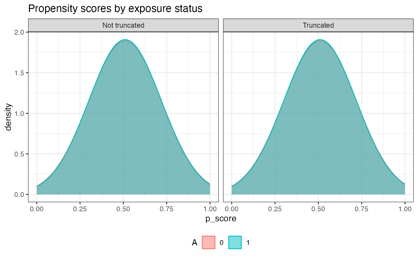
`plot.p_score()`	Plot the propensity scores by exposure status	plot.p_score
`plot.ip_weights()`	Plot the inverse probability weights using truncated propensity scores	plot.ip_weights

Public Variables

Variable	Generated by	Return
`n`	Constructor	Number of observations
`stratified_fitted`	`stratified_fit()`	Fit the outcome model stratified by exposure status
`obs_est`	`fit()` & `summary()`	Components calculating average causal effects
`estimates`	`summary()`	A list of Risk difference, risk ratio, odds ratio
`result`	`summary()`	A matrix contains RD, ATT, ATC, RR and OR with their SE and 95%CI
`g.plot`	`plot.p_score()`	A density plot of propensity scores by exposure status
`ip_weights.plot`	`plot.ip_weights()`	A box plot of inverse probability weights
`libs`	`fit()`	SuperLearner or sl3 libraries and their fitted objects
`sl.fit`	Constructor	A wrapper function for fitting SuperLearner or sl3
`sl.predict`	Constructor	A wrapper function using `sl.fit` to predict

Public Variable Details

stratified_fit: An indicator for whether the outcome model is fitted stratified by exposure status in the fit() method. Only when using stratified_fit() to turn on stratified_fit = TRUE, summary outputs average treatment effects among the treated and the controls.
obs_est: After using fit() and summary() methods, this list contains the propensity scores (p_score), counterfactual predictions (mu, mu1 & mu0) and efficient influence functions (aipw_eif1 & aipw_eif0) for later average treatment effect calculations.
g.plot: This plot is generated by ggplot2::geom_density
ip_weights.plot: This plot uses truncated propensity scores stratified by exposure status (ggplot2::geom_boxplot)

References

Zhong Y, Kennedy EH, Bodnar LM, Naimi AI (2021). AIPW: An R Package for Augmented Inverse Probability Weighted Estimation of Average Causal Effects. American Journal of Epidemiology.

Robins JM, Rotnitzky A (1995). Semiparametric efficiency in multivariate regression models with missing data. Journal of the American Statistical Association.

Chernozhukov V, Chetverikov V, Demirer M, et al (2018). Double/debiased machine learning for treatment and structural parameters. The Econometrics Journal.

Kennedy EH, Sjolander A, Small DS (2015). Semiparametric causal inference in matched cohort studies. Biometrika.

Examples

library(SuperLearner)
#> Loading required package: nnls
#> Loading required package: gam
#> Loading required package: splines
#> Loading required package: foreach
#> Loaded gam 1.22-2
#> Super Learner
#> Version: 2.0-28.1
#> Package created on 2021-05-04
library(ggplot2)

#create an object
aipw_sl <- AIPW$new(Y=rbinom(100,1,0.5), A=rbinom(100,1,0.5),
                    W.Q=rbinom(100,1,0.5), W.g=rbinom(100,1,0.5),
                    Q.SL.library="SL.mean",g.SL.library="SL.mean",
                    k_split=1,verbose=FALSE)

#fit the object
aipw_sl$fit()
# or use `aipw_sl$stratified_fit()` to estimate ATE and ATT/ATC

#calculate the results
aipw_sl$summary(g.bound = 0.025)

#check the propensity scores by exposure status after truncation
aipw_sl$plot.p_score()